
一、概述
日常生活中,我们能用到的扫描全能王、美图秀秀、PhotoShop等软件,均是数字图像处理的应用工具,如果对图像处理有较高要求,就需要深入学习数字图像处理,用高级语言及各种复杂算法来处理图像了。
数字图像处理的本质是对图像的数字化表示(像素矩阵)进行有目的的变换,对像素矩阵进行数值操作 ,提取有用的信息或优化视觉效果。
一副图像可以定义为一个二维离散函数f(x, y),其中(x, y)是图像中的一个像素点的坐标,而f是该点的强度值/灰度值(对于灰度图,是亮度;对于彩色图,通常是红、绿、蓝三个通道的强度值),所有的处理都是对这个函数进行数学运算。其中,当x,y,f为有限的离散量时,称该图像为数字图像。
数字图像处理的目的如下:
改善视觉效果:使图像看起来更清晰、更漂亮,如锐化、去噪、对比度增强、彩色化、修复老照片等;
便于机器分析:为后续的自动识别做准备:例如边缘检测、图像分割;
信息提取与理解:从图像中获取我们关心的数据,如医学影像检测肿瘤大小、人脸识别识别身份、对图像进行计数等;
高效存储与传输:对图像进行压缩,减少存储空间和网络带宽的占用,如:JPEG、PNG格式;
二、学习路径
1、参考教材:冈萨雷斯的《数字图像处理》
2、b站up主:
本篇文章主要基于b站:“十四阿哥很nice”的“手写图像处理库”系列视频进行学习和总结(该系视频是结合冈萨雷斯的《数字图像处理》第三章内容的实践部分),可惜up主只更新了5个视频之后就断更了~~~
俗话说,理论需要结合实践,虽然视频不是很全,还是先开动吧。
三、学习案例
3.1反色变换、对数变换
1、应用场景
反色变换和对数变换是为了:调整图像的亮度和灰度分布,解决原始图像“细节隐藏”或“动态范围不匹配”的问题,应用场景:文档、扫描件处理、医学影像增强等。
2、原理解释
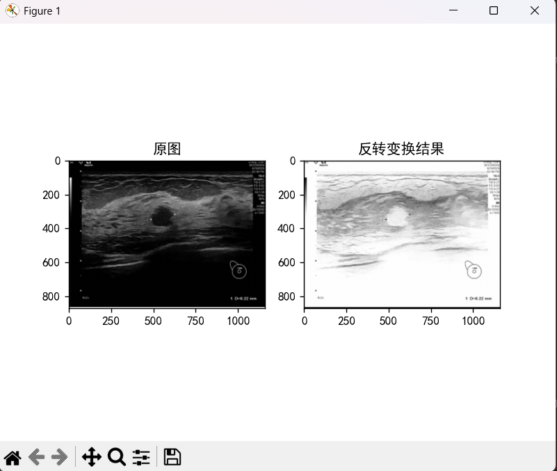
反色变换:将图像中每个像素的亮度值反转,本质是对像素值做“最大值减去原像素值”的运算。若对于彩色图像(如 RGB/BGR),其反色是对每个通道的像素分别作反色运算。
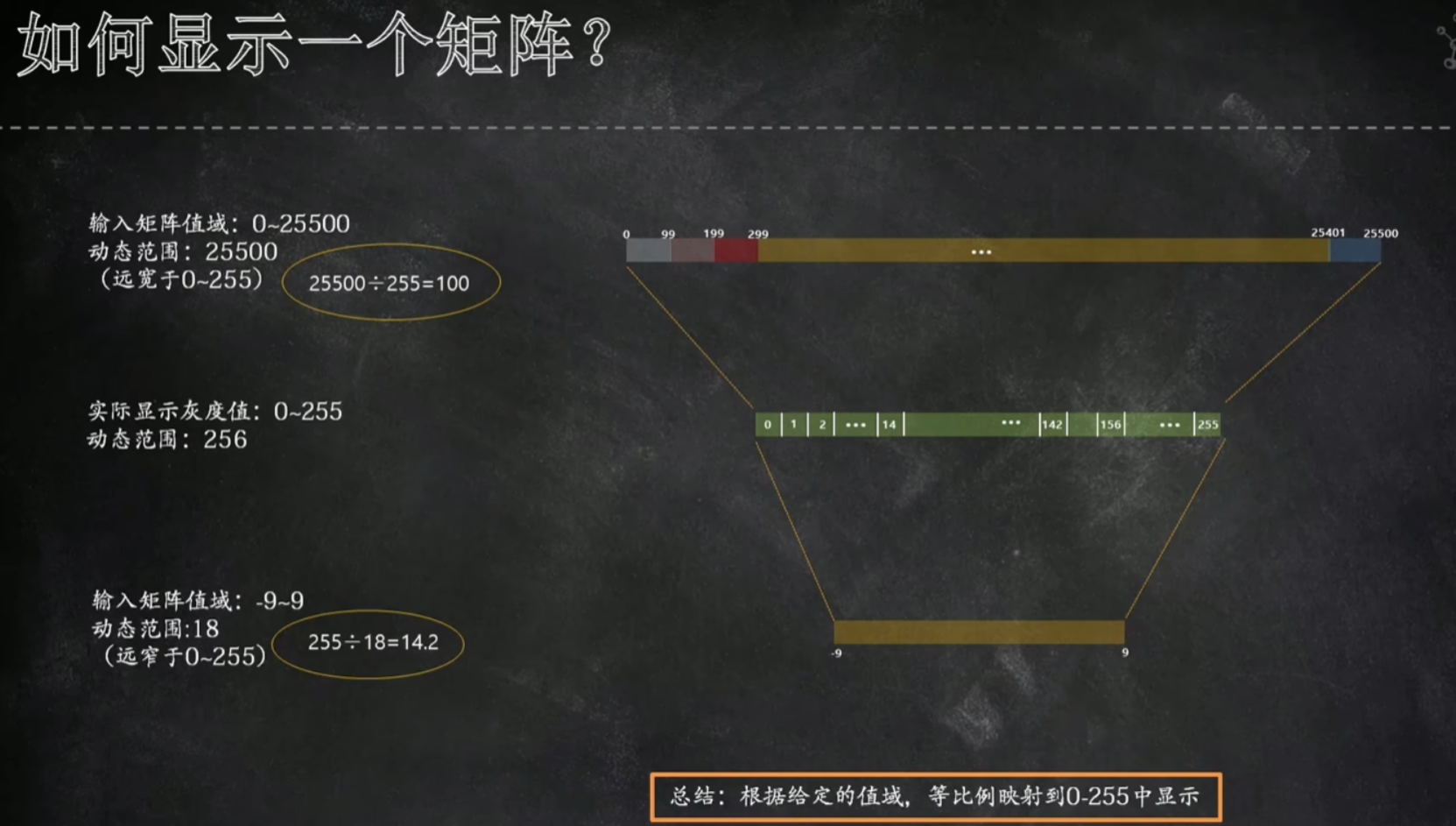
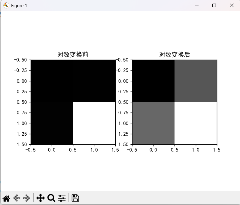
对数变换:可以让图像显示更多细节,主要是为了压缩值域动态范围,从而让动态范围过宽的图像可以显示更多肉眼可见的细节。
tips:对于单通道的图像,其灰度值范围在0~255,其中0为纯黑,255为纯白。
如果给定矩阵的值域为0~25500或是-9~9,则我们需要将值域等比例映射至0~255的区间内,才能清晰看到图像。
3、实践
1)反转变换
import numpy as np
from PIL import Image
import matplotlib  # 导入主模块
matplotlib.use('TkAgg')  # 切换 Matplotlib 后端,解决 PyCharm 兼容性问题方法,切换到 Tkinter 后端(需保证 Python 安装了 tkinter,通常默认有),正确调用 use()
import matplotlib.pyplot as plt

# 解决中文显示问题
# plt.rcParams["font.family"] =  ["Microsoft YaHei", "SimSun", "SimHei"]  # 这三种字体 Windows 默认都有
# plt.rcParams["axes.unicode_minus"] = False

print("安装成功!")  # 无报错则说明安装成功
def set_Chinese():   # 中文显示工具函数
    # rcParams 本质是 matplotlib 主模块的全局配置字典
    matplotlib.rcParams["font.sans-serif"] =["SimHei"]
    matplotlib.rcParams["axes.unicode_minus"]=False

def image_inverse(input):
    value_max = np.max(input) #求输入图像最大灰度值
    output = value_max - input
    return output;

if __name__ == "__main__":
    # 用举矩阵测试反转
    # input = np.array([[0,20,160],[45,50,100],[100,45,30]])
    # output = image_inverse(input)
    # print(output)

    # 用图片测试反转
    set_Chinese()
    gray_image = np.asarray(Image.open("B_chao.jpg").convert('L'))
    inv_img = image_inverse(gray_image)

    fig = plt.figure() #创建 matplotlib 绘图窗口
    ax1 = fig.add_subplot(121) #在 fig 窗口中添加一个 “子图区域”,参数 121 是 “行 × 列 × 子图序号” 的缩写
    ax1.set_title('原图')
    ax1.imshow(gray_image, cmap='gray', vmin=0, vmax=255)

    ax2 = fig.add_subplot(122)
    ax2.set_title('反转变换结果')
    ax2.imshow(inv_img, cmap='gray', vmin=0, vmax=255)

    plt.show()
运行结果
2)对数变换
import numpy as np
import matplotlib  # 导入主模块
matplotlib.use('TkAgg')  # 切换 Matplotlib 后端,解决 PyCharm 兼容性问题方法,切换到 Tkinter 后端(需保证 Python 安装了 tkinter,通常默认有),正确调用 use()
import matplotlib.pyplot as plt

# 中文显示工具函数
def set_Chinese():
    # rcParams 本质是 matplotlib 主模块的全局配置字典
    matplotlib.rcParams["font.sans-serif"] =["SimHei"]
    matplotlib.rcParams["axes.unicode_minus"]=False

def image_log(input):
    return np.log(input+1)

if __name__ == "__main__":
    set_Chinese()
    # input = np.array([[-9,-8],[1,2]])
    input = np.array([[10, 150], [250, 25500]])

    output = image_log(input)
    print(output)

    fig = plt.figure()
    ax1 = fig.add_subplot(121)
    ax1.set_title("对数变换前")
    # ax1.imshow(input,cmap='gray',vmin=-9,vmax=9)
    ax1.imshow(input, cmap='gray', vmin=0, vmax=25500)

    ax2= fig.add_subplot(122)
    ax2.set_title("对数变换后")
    ax2.imshow(output, cmap='gray') #不加 vmin/vmax:自动适配数组的实际范围,可能增强对比度(适合非标准范围的图像)。

    plt.show()
运行结果
3.2伽马变换
1、原理解释
伽马变换:基于幂函数的非线性灰度变换,核心作用是调整图像的亮度和对比度,尤其是修正设备特性导致的亮度偏差,或者增强图像中的暗部、高光细节。
gamma变换之所以能调节图像的对比度,本质原因:它能对输入图像不同灰度区间的动态范围,做相对独立的调整。
gamma曲线的特性如下: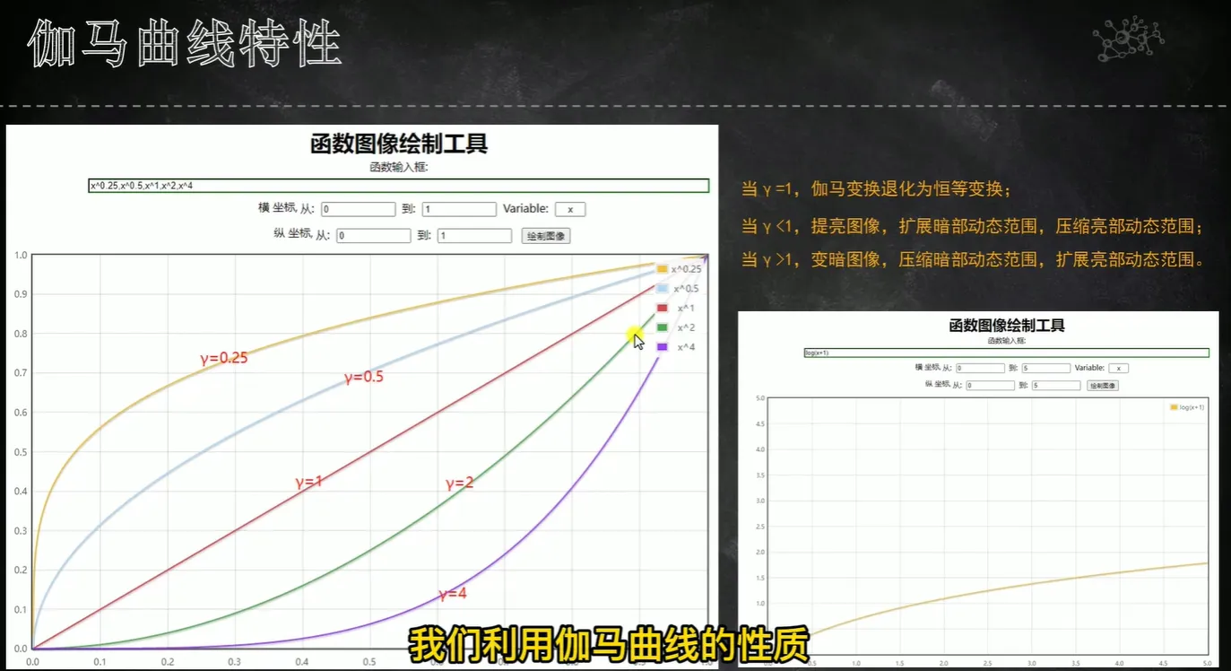
当gamma<1,提亮图像,扩展暗部动态范围,压缩亮部动态范围(小灰度区间被扩大,大灰度区间被缩小)
当gamma>1,变暗图像,压缩暗部动态范围,扩展亮部动态范围(小灰度区间被缩小,大灰度区间被扩大)


2、实践
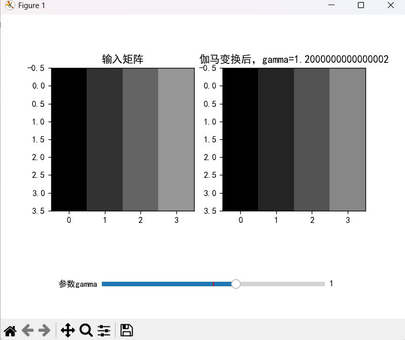
1)ganmma变换
import numpy as np
from PIL import Image
import matplotlib  # 导入主模块
matplotlib.use('TkAgg')
import matplotlib.pyplot as plt
from matplotlib.widgets import Slider, Button, RadioButtons

def set_Chinese():   # 中文显示工具函数
    # rcParams 本质是 matplotlib 主模块的全局配置字典
    matplotlib.rcParams["font.sans-serif"] =["SimHei"]
    matplotlib.rcParams["axes.unicode_minus"]=False

def gamma_trans(input,gamma=2,eps=0):
    return 255.*(((input+eps)/255.)**gamma)

def update_gamma(val):
    gamma=slider1.val
    output=gamma_trans(input_arr, gamma=gamma, eps=0)
    print("-------------\n",output)
    # 因为输出矩阵随时更新,频繁刷新,所以输出图像显示代码写在回调函数中
    ax1.set_title("伽马变换后,gamma="+str(gamma))
    ax1.imshow(output, cmap='gray', vmin=0, vmax=255)

if __name__ == "__main__":
    set_Chinese()

    input_arr = np.array([[0,50,100,150],
                         [0,50,100,150],
                         [0,50,100,150],
                         [0,50,100,150]])

    fig = plt.figure()
    ax0 = fig.add_subplot(121)
    ax0.set_title("输入矩阵")
    ax0.imshow(input_arr, cmap='gray', vmin=0, vmax=255)

    ax1 = fig.add_subplot(122)

    # 往显示主体添加滑动条
    plt.subplots_adjust(bottom=0.3) #为滑动条预留出足够的显示空间。
    s1 = plt.axes([0.25, 0.1, 0.55, 0.03],facecolor='lightgoldenrodyellow')
    slider1 = Slider(s1, '参数gamma', 0.0, 2.0, valfmt='%.f', valinit=1.0, valstep=0.1)
    slider1.on_changed(update_gamma) #绑定滑动条的回调函数
    slider1.reset #滑动条的重置操作
    slider1.set_val(1) #滑动条的重置操作

    plt.show()
运行结果
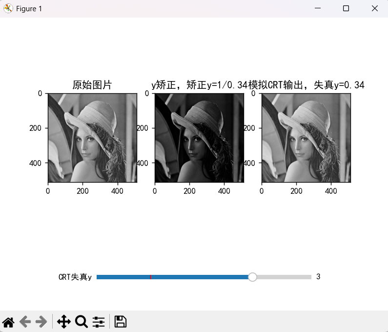
2)ganmma变换-crt
import numpy as np
from PIL import Image
import matplotlib  # 导入主模块
matplotlib.use('TkAgg')
import matplotlib.pyplot as plt
from matplotlib.widgets import Slider, Button, RadioButtons

def set_Chinese():   # 中文显示工具函数
    # rcParams 本质是 matplotlib 主模块的全局配置字典
    matplotlib.rcParams["font.sans-serif"] =["SimHei"]
    matplotlib.rcParams["axes.unicode_minus"]=False

def gamma_trans(input,gamma=2,eps=0):
    return 255.*(((input+eps)/255.)**gamma)

def crt_distortion(input,gamma=2,eps=0): #模拟crt失真
    return 255.*((input/255.)**gamma)

def update_gamma(val):
    gamma=slider1.val

    #需要先对图像进行预处理(根据y),预处理过程在crt输出前,做一个失真1/y的运算----图像送入CRT前,先做y变换处理
    gamma=1/gamma
    correct_img = gamma_trans(gray_img, 1/gamma,0)
    ax1.set_title("y矫正,矫正y=1/"+str(round(gamma,2)))
    ax1.imshow(correct_img,cmap='gray', vmin=0, vmax=255)

    # 简易模拟crt输出
    output=crt_distortion(correct_img, gamma)
    print(output)
    ax2.set_title("模拟CRT输出,失真y="+str(round(gamma,2))) #round方法可以使gamma只显示小数点后两位
    ax2.imshow(output, cmap='gray', vmin=0, vmax=255)

if __name__ == "__main__":
    set_Chinese()

    gray_img = np.asanyarray(Image.open("./lena.jpg").convert('L'))

    fig = plt.figure()
    ax0 = fig.add_subplot(131)
    ax1 = fig.add_subplot(132)
    ax2 = fig.add_subplot(133)

    ax0.set_title("原始图片")
    ax0.imshow(gray_img, cmap='gray', vmin=0, vmax=255)

    # 往显示主体添加滑动条
    plt.subplots_adjust(bottom=0.3) #为滑动条预留出足够的显示空间。
    s1 = plt.axes([0.25, 0.1, 0.55, 0.03],facecolor='lightgoldenrodyellow')
    slider1 = Slider(s1, 'CRT失真y', 0.0, 4.0, valfmt='%.f', valinit=1.0, valstep=0.1)
    slider1.on_changed(update_gamma) #绑定滑动条的回调函数
    slider1.reset #滑动条的重置操作
    slider1.set_val(2) #滑动条的重置操作

    plt.show()
运行结果
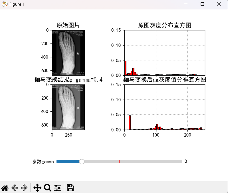
3)ganmma变换-增加对比度
import numpy as np
from PIL import Image
import matplotlib  # 导入主模块
matplotlib.use('TkAgg')
import matplotlib.pyplot as plt
from matplotlib.widgets import Slider, Button, RadioButtons

def set_Chinese():   # 中文显示工具函数
    # rcParams 本质是 matplotlib 主模块的全局配置字典
    matplotlib.rcParams["font.sans-serif"] =["SimHei"]
    matplotlib.rcParams["axes.unicode_minus"]=False

def gamma_trans(input,gamma=2,eps=0):
    return 255.*(((input+eps)/255.)**gamma)

def update_gamma(val):
    #获取滑块数值,做y
    gamma=slider1.val
    output=gamma_trans(gray_img, gamma, 0.2)

    #显示y变换结果图像
    ax3.clear()
    ax3.set_title("伽马变换结果,gamma="+str(round(gamma, 2)))
    ax3.imshow(output,cmap='gray', vmin=0, vmax=255)
    #显示y变换结果图像的灰度分布直方图
    ax4.clear()
    ax4.set_xlim(0, 255)  # 设置x轴分布范围
    ax4.set_ylim(0, 0.15)  # 设置y轴分布范围
    ax4.grid(True, linestyle=":", linewidth=1)
    ax4.set_title("伽马变换后,灰度值分布直方图", fontsize=12)
    ax4.hist(output.flatten(), bins=50, density=True, color='r', edgecolor='k')  # 调用hist直接获

if __name__ == "__main__":
    set_Chinese()

    gray_img = np.asanyarray(Image.open("./DRfeet.png").convert('L'))

    fig = plt.figure()
    ax1 = fig.add_subplot(221)
    ax2 = fig.add_subplot(222)
    ax3 = fig.add_subplot(223)
    ax4 = fig.add_subplot(224)

    # ax1显示原图
    ax1.set_title("原始图片")
    ax1.imshow(gray_img, cmap='gray', vmin=0, vmax=255)

    # ax2显示原图的灰度分布直方图
    ax2.grid(True, linestyle=":", linewidth=1)
    ax2.set_title("原图灰度分布直方图", fontsize=12)
    ax2.set_xlim(0, 255) #设置x轴分布范围,x 轴:代表灰度值(0~255,0 = 黑,255 = 白)
    ax2.set_ylim(0, 0.15)  # 设置y轴分布范围,y 轴:代表 “像素在该灰度区间的频率密度”(因 density=True,表示该区间像素数占总像素数的比例)
    ax2.hist(gray_img.flatten(), bins=50, density=True, color='r', edgecolor='k')

    # 往显示主体下方添加滑动条
    plt.subplots_adjust(bottom=0.3)  # 为滑动条预留出足够的显示空间。
    s1 = plt.axes([0.25, 0.1, 0.55, 0.03],
                  facecolor='lightgoldenrodyellow')
    slider1 = Slider(s1, '参数gamma', 0.0, 2.0, valfmt='%.f', valinit=1.0,
                     valstep=0.1)
    slider1.on_changed(update_gamma)  # 绑定滑动条的回调函数
    slider1.reset  # 滑动条的重置操作
    slider1.set_val(1.0)  # 滑动条的重置操作

    plt.show()
运行结果
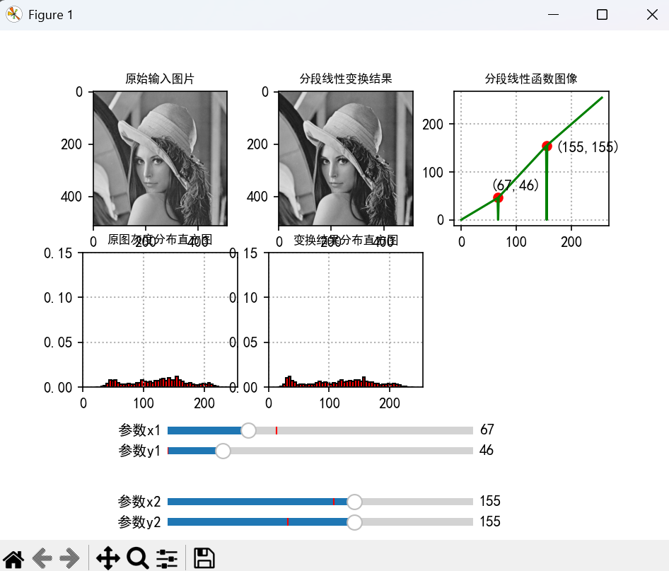
3.3分段变换
1、原理解释
分段变换是一种“按区间定义不同映射规则”的数值方法,核心是对数据的不同范围做针对性调整。

假若衣服图像的灰度值恰好落在如图所示的这段曲线内,动态范围只会产生微弱的变化,无法产生肉眼可感知的对比度变换
伽马变换:斜率大于1的区间,扩展灰度动态范围;斜率小于1的区间,压缩灰度动态范围;
幂函数的问题:曲线中有一个点的斜率为1,就会造成在1附近的这段曲线,无法有效改变图像动态范围
由此引出:分段变换---精准控制不同区间的数值映射,设配具体场景的需求。
2、实践
import numpy as np
from PIL import Image
import matplotlib.pyplot as plt
from matplotlib.widgets import Slider
import matplotlib  # 导入主模块
matplotlib.use('TkAgg')

def set_Chinese():   # 中文显示工具函数
    # rcParams 本质是 matplotlib 主模块的全局配置字典
    matplotlib.rcParams["font.sans-serif"] =["SimHei"]
    matplotlib.rcParams["axes.unicode_minus"]=False


#三段对比度拉伸变换,其中x1,y1和x2,y2为分段点
def three_linear_transformation(x,x1,y1,x2,y2): #x是输入矩阵
    #1、检查参数,避免分母为0
    if x1==x2 or x2 == 255:
        print("[INFO] x1=%d,x2=%d -> 调用词函数必须满足x1!=x2且x2!=255]" %(x1,x2))
        return None

    #2、执行分段线性变换
    m1=(x<x1) #比较运算,当x<x1时,置1,否则置0
    m2=(x1 <= x)&(x <= x2) #注意这里要用&,且注意运算顺序
    m3=(x>x2)
    out = (y1/x1*x)*m1 \
            +((y2-y1)/(x2-x1)*(x-x1)+y1)*m2 \
             +((255-y2)/(255-x2)*(x-x2)+y2)*m3

    #3、获取分段线性函数的点集,用于绘制函数图像
    # 这段代码的核心是通过布尔掩码过滤和分段函数计算
    x_point = np.arange(0,256,1)
    cond2=[True if(i>x1 and i<x2) else False for i in x_point]
    y_point = (y1/x1*x_point)*(x_point<x1) \
                +((y2-y1)/(x2-x1)*(x_point-x1)+y1)*cond2 \
                +((255-y2)/(255-x2)*(x_point-x2)+y2)*(x_point>x2)
    return out, x_point, y_point

def update_trans(val):
    #读入4个滑动条的值
    x1,y1 = slider_x1.val,slider_y1.val
    x2,y2 = slider_x2.val,slider_y2.val

    #执行分段线性变换
    out,x_point,y_point =three_linear_transformation(gray_img,x1,y1,x2,y2)

    #绘制变换结果图像
    ax2.clear()
    ax2.set_title("分段线性变换结果", fontsize=8)
    ax2.imshow(out, cmap='gray', vmin=0, vmax=255)

    #绘制函数图像
    ax3.clear()
    ax3.annotate('(%d,%d)'%(x1,y1),xy=(x1,y1),xytext=(x1-15,y1+15))
    ax3.annotate('(%d,%d)'%(x2,y2),xy=(x2,y2),xytext=(x2+15,y2-15))
    ax3.set_title("分段线性函数图像", fontsize=8)
    ax3.grid(True, linestyle=':', linewidth=1)
    ax3.plot([x1,x2], [y1,y2], 'ro')
    ax3.plot(x_point, y_point, 'g')

    # 显示变换结果的灰度分布直方图
    ax5.clear()
    ax5.grid(True, linestyle=':', linewidth=1)
    ax5.set_title("变换结果分布直方图", fontsize=8)
    ax5.set_xlim(0, 255)  # 设置x轴分布范围
    ax5.set_ylim(0, 0.15)  # 设置y轴分布范围
    ax5.hist(out.flatten(), bins=50, density=True, color='r', edgecolor='k')  # 调用hist直接获

#主函数
if __name__ == "__main__":
    set_Chinese()
    #以灰度值方式读取图像,
    gray_img = np.asanyarray(Image.open("../day2/lena.jpg").convert('L'))
    print("[INFO]原图尺寸为:",gray_img.shape)

    #创建一个显示主体,并分成五个显示区域
    fig = plt.figure()
    ax1 = fig.add_subplot(231)
    ax2 = fig.add_subplot(232)
    ax3 = fig.add_subplot(233)
    ax4 = fig.add_subplot(234)
    ax5 = fig.add_subplot(235)

    #显示原图及灰度分布直方图
    ax1.set_title("原始输入图片", fontsize=8)
    ax1.imshow(gray_img,cmap='gray',vmin=0,vmax=255)

    ax4.grid(True, linestyle=':',linewidth=1)
    ax4.set_title('原图灰度分布直方图',fontsize=8)
    ax4.set_xlim(0, 255)  # 设置x轴分布范围
    ax4.set_ylim(0, 0.15)  # 设置y轴分布范围
    ax4.hist(gray_img.flatten(), bins=50, density=True, color='r', edgecolor='k')  # 调用hist直接获

    #创建四个滑动条,用于调节x1,x2,y1,y2四个值
    plt.subplots_adjust(bottom=0.3)
    x1 = plt.axes([0.25, 0.2, 0.45, 0.03],facecolor='lightgoldenrodyellow')
    slider_x1 = Slider(x1, '参数x1', 0.0, 255., valfmt='%.f', valinit=91,valstep=1)
    slider_x1.on_changed(update_trans)

    y1 = plt.axes([0.25, 0.16, 0.45, 0.03], facecolor='lightgoldenrodyellow')
    slider_y1 = Slider(y1, '参数y1', 0.0, 255., valfmt='%.f', valinit=0, valstep=1)
    slider_y1.on_changed(update_trans)

    x2 = plt.axes([0.25, 0.06, 0.45, 0.03], facecolor='white')
    slider_x2 = Slider(x2, '参数x2', 0.0, 254., valfmt='%.f', valinit=138, valstep=1)
    slider_x2.on_changed(update_trans)

    y2 = plt.axes([0.25, 0.02, 0.45, 0.03], facecolor='lightgoldenrodyellow')
    slider_y2 = Slider(y2, '参数y2', 0.0, 254., valfmt='%.f', valinit=100, valstep=1)
    slider_y2.on_changed(update_trans)

    update_trans(None)
    plt.show()
运行结果
3.4直方图均衡化
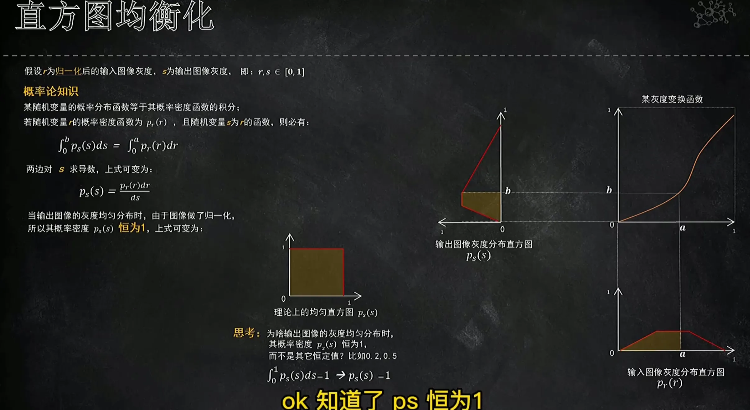
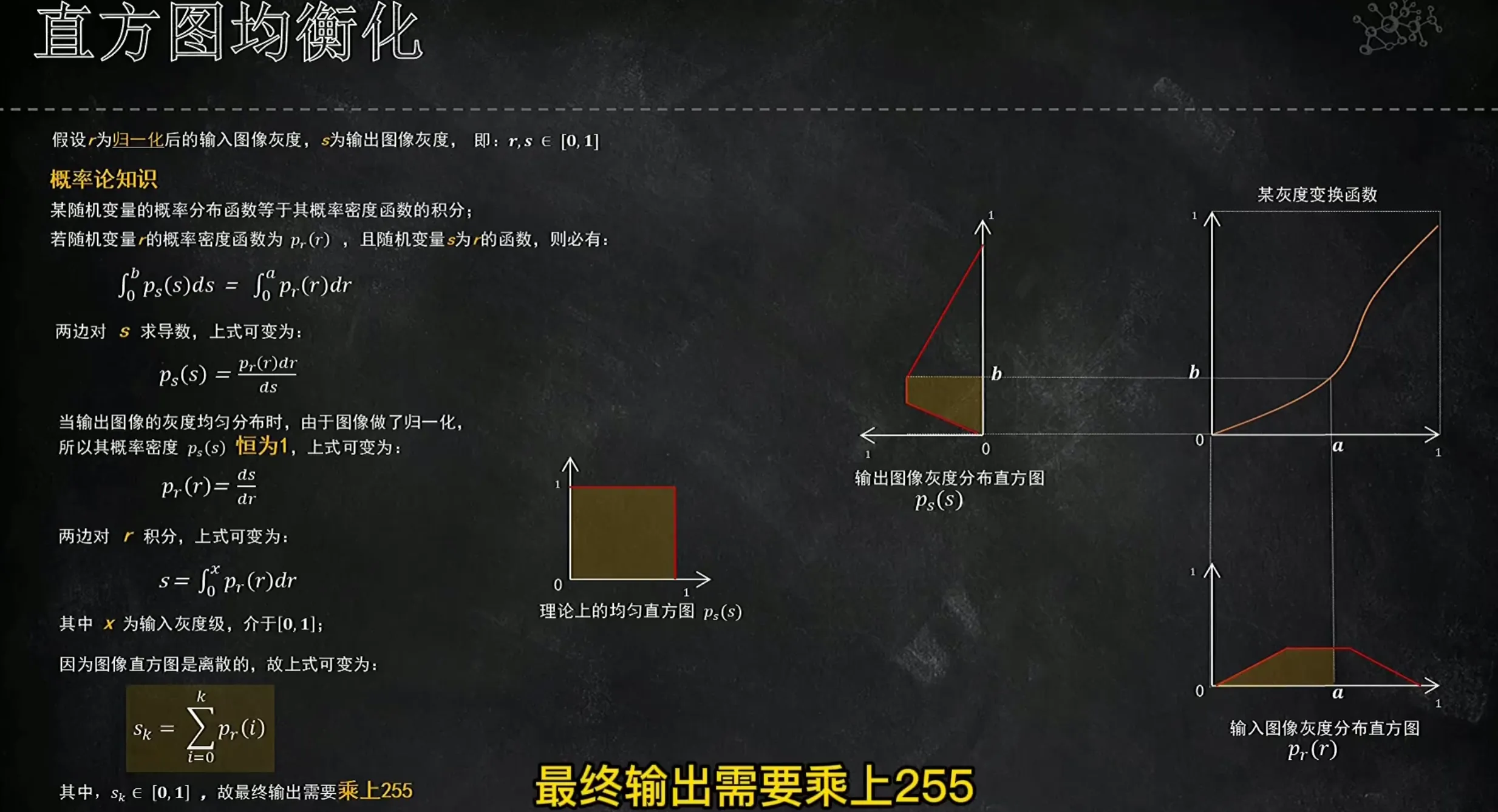
1、原理解释
直方图均衡化:核心是通过调整图像的灰度分布,让原本集中在某一区间的灰度值均匀分布到整个灰度范围(通常为0~255),从而提升图像细节。
图像的灰度直方图:统计每个灰度值(0~255)在图像中出现的次数(频次),很坐标是灰度值,纵坐标是频次
均衡化的目标:把“集中型”直方图变为均匀型直方图——让每个回去区间像素量尽可能均衡
实现原理:通过累积分布函数(CDF)讲原始灰度值映射到新的灰度值,拉伸密集区间、压缩稀疏区间,最终扩大灰度动态范围。
2、实践
import numpy as np
from PIL import Image
import matplotlib.pyplot as plt
from matplotlib.widgets import Slider
import matplotlib # 导入主模块
matplotlib.use('TkAgg')
# 中文显示工具函数
def set_Chinese():
# rcParams 本质是 matplotlib 主模块的全局配置字典
matplotlib.rcParams["font.sans-serif"] =["SimHei"]
matplotlib.rcParams["axes.unicode_minus"]=False
#获取图像的概率密度
def get_pdf(in_img):
total = in_img.shape[0]*in_img.shape[1] #计算图片总像素数
return [np.sum(in_img == i)/total for i in range(256)] #求概率密度,#掩码举证就是由True和False组成的和im_img同形状的矩阵
#直方图均衡化(核心代码)
def hist_equal(in_img):
#1、求输入图像的概率密度
Pr = get_pdf(in_img)
#2、构造输出图像(初始化成输入)
out_img = np.copy(in_img)
#3、执行“直方图均衡化”(执行累积分布函数变换)
y_points = []#存储点集,用于画图
SUMK =0. #累加值存储变量
for i in range(256):
SUMK = SUMK +Pr[i] #SUMK 是从灰度 0 到灰度 i 的所有概率之和,范围在 0~1 之间。
out_img[(in_img ==i)] = SUMK*255. #灰度值归一化 ,灰度值映射(SUMK * 255):将累积概率(0~1)缩放至 0~255 的灰度范围,得到新的灰度值。“原始图像中所有灰度为 i 的像素,在输出图像中统一更新为新映射值”
y_points.append(SUMK*255.) #构造绘制函数图像的点集,y_points 存储每个原始灰度 i 对应的新灰度值
return out_img,y_points
if __name__ == "__main__":
set_Chinese()
# 以灰度值方式读取图像,
#gray_img = np.asanyarray(Image.open("../day2/lena.jpg").convert('L'))
gray_img = np.asanyarray(Image.open("./planet.png").convert('L'))
#对原图执行直方图均衡化
out_img,y_points =hist_equal(gray_img)
#创建一个显示主体,并分成6个显示区域
fig = plt.figure()
ax1,ax2=fig.add_subplot(231),fig.add_subplot(232)
ax3, ax4 = fig.add_subplot(234), fig.add_subplot(235)
ax5 = fig.add_subplot(236)
#窗口显示:原图,原图灰度分布,结果图像,结果图像灰度分布
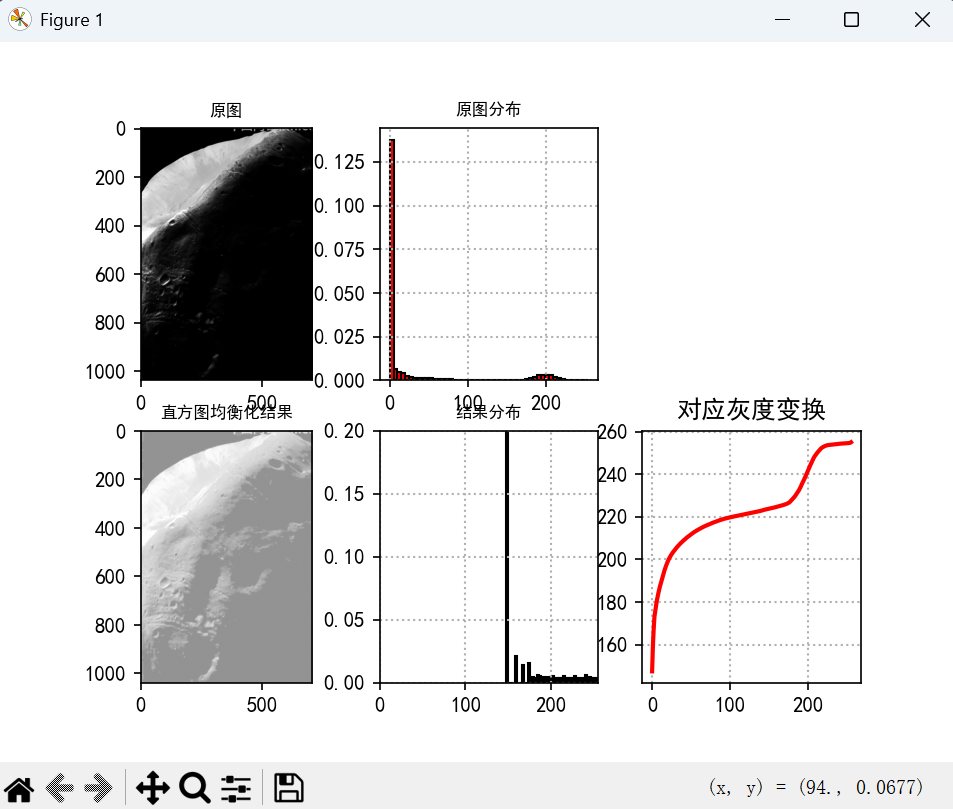
ax1.set_title("原图",fontsize = 8)
ax1.imshow(gray_img,cmap='gray',vmin=0,vmax=255)
ax2.grid(True,linestyle=':', linewidth = 1)
ax2.set_title("原图分布", fontsize=8)
ax2.hist(gray_img.flatten(),bins=50,density=True,color='r',edgecolor='k') #将多维数组(如二维图像数组)“展平” 为一维数组,即将所有元素按顺序排列成一个连续的序列。
ax3.set_title("直方图均衡化结果",fontsize = 8)
ax3.imshow(out_img,cmap='gray',vmin=0,vmax=255)
ax4.grid(True,linestyle=':', linewidth = 1)
ax4.set_title("结果分布",fontsize = 8)
ax4.set_xlim(0,255) #设置x轴分布范围
ax4.set_ylim(0,0.2) #设置y轴分布范围
ax4.hist(out_img.flatten(),bins=50,density=True,color='r',edgecolor='k')
#窗口显示:绘制对应的灰度变换函数
ax5.set_title("对应灰度变换",fontsize=12)
ax5.grid(True,linestyle=':', linewidth = 1)
ax5.plot(np.arange(0, 256, 1),y_points,color='r',lw=2) #np.arange(0,256,1)
ax5.text(25,70,r'$s_k=255\times\sum_{i=0}^{k}p_r(i)$',fontsize=9)
plt.show()运行结果
3.5直方图规定化
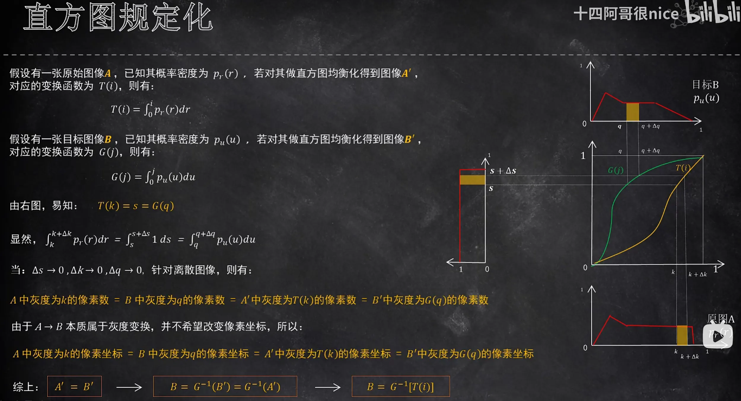
1、原理解释
直方图规定化:让一副图像的灰度分布,主动”模仿“另一副目标图像的灰度分布的技术
简单来说:借目标图的直方图形状,改变原图的灰度分布,最终让原图的视觉风格、对比度和目标图趋于一致。
直方图均衡化:目标是 “均匀分布”(固定目标),不管原始图像是什么样,都往 “灰度值铺满 0-255” 的方向调整。
直方图规定化:目标是 “自定义分布”(目标由你选),比如想让图 A 的直方图长得和图 B 一样,就以图 B 为 “模板”,调整图 A 的灰度。
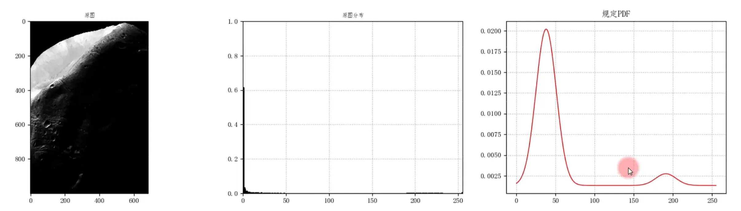
使用直方图均衡化的问题如下:把0处的峰值矫正到155附近,修正图像无法保持原有色调,原因:由于超灰度区间的概率密度过大,导致变换函数直接呈现“阶跃”。

因此设想,想要实现如下图的灰度分布直方图变换 ------使用直方图规定化
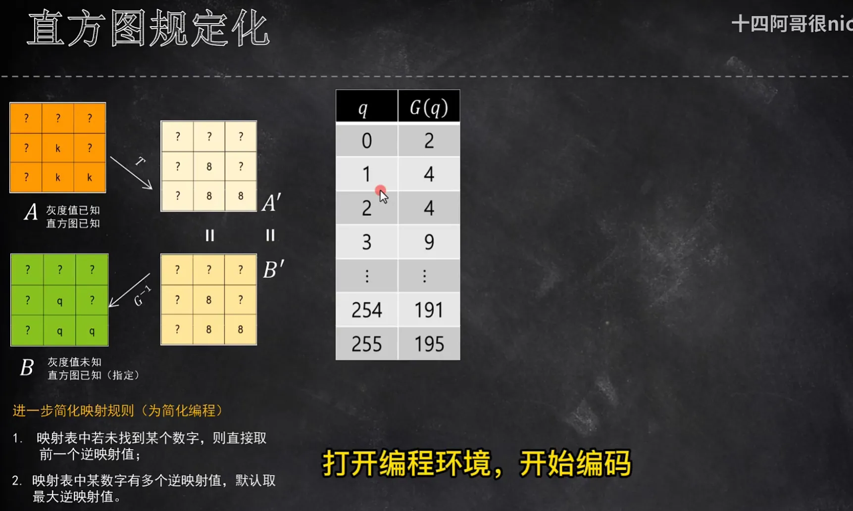
把0-255共256个数送进变换函数G,得到灰色的表格
2、实践
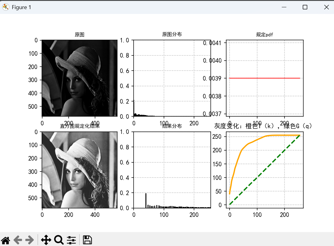
1)直方图规定化:均匀分布
import numpy as np
from PIL import Image
import matplotlib.pyplot as plt
from matplotlib.widgets import Slider
import matplotlib  # 导入主模块
matplotlib.use('TkAgg')  # 切换 Matplotlib 后端,解决 PyCharm 兼容性问题方法,切换到 Tkinter 后端(需保证 Python 安装了 tkinter,通常默认有),正确调用 use()

# 中文显示工具函数
def set_Chinese():
    # rcParams 本质是 matplotlib 主模块的全局配置字典
    matplotlib.rcParams["font.sans-serif"] =["SimHei"]
    matplotlib.rcParams["axes.unicode_minus"]=False

#获取图像的概率密度
def get_pdf(in_img):
    total = in_img.shape[0] * in_img.shape[1] #计算图像的总像素数
    return [ np.sum(in_img == i)/total for i in range(256) ] #求概率密度

#直方图均衡化(核心代码)
def hist_equal(in_img):
    #1、求原始图像的概率密度
    Pr = get_pdf(in_img)

    #2、构造输出图像(初始化成输入)
    out_img = np.copy(in_img)

    #3、执行“直方图均衡化”(执行累积分布函数变换)
    y_points = [] #存储点集,用于画图
    SUMk = 0 #累加值存储变量
    for i in range(256):
        SUMk = SUMk + Pr[i]  # SUMK 是从灰度 0 到灰度 i 的所有概率之和,范围在 0~1 之间。
        out_img[(in_img == i)] = SUMk * 255 # 灰度值归一化 ,灰度值映射(SUMK * 255):将累积概率(0~1)缩放至 0~255 的灰度范围,得到新的灰度值。“原始图像中所有灰度为 i 的像素,在输出图像中统一更新为新映射值”
        y_points.append(SUMk * 255)  # 构造绘制函数图像的点集,y_points 存储每个原始灰度 i 对应的新灰度值
    return out_img.astype("int32"), y_points

#生成均匀分布
def gen_eq_pdf():
    return [ 0.0039 for i in range(256)] #均匀概率密度1/256 = 0.0039

#构造目标图像的映射表(核心代码)
def gen_target_table(Pv):
    table = []
    SUMq = 0.
    for i in range(256):
        SUMq = SUMq + Pv[i]
        table.append(round(SUMq*255, 0)) #四舍五入
    return table

#直方图规定化(核心代码)
def hist_specify(in_img=None):
    #1、拿到目标图像规定的概率密度,并构造映射表
    Pv = gen_eq_pdf()#均匀分布, 假设生成均匀分布的PDF(目标分布)
    table = gen_target_table(Pv) # 目标分布的累积映射表
    print(table)

    #2、对原始图像做直方图均衡
    ori_eq_img, T_points = hist_equal(in_img) # 得到中间均衡化图像,ori_eq_img是原始图像经过直方图均衡化后的结果(灰度分布已被拉伸为近似均匀分布)

    #3、构造输出图像(初始化成输入)
    out_img = np.copy(ori_eq_img)

    #4、执行“直方图规定化”(做逆映射B'->B)
    mal_val = 0 #逆映射值初始化为0
    for v in range(256):
        if v in ori_eq_img: #存在于B’,如果当前灰度v存在于均衡化图像中
            if v in table: #存在于映射表,如果当前灰度v在目标映射表中存在对应值
#拿到指定值最后出现的索引,python数组中的index下标只能拿到最小下标,多以要将table数组颠倒,再来拿下标,相当于拿到最大下标
                mal_val = len(table) - table[::-1].index(v)-1
            out_img[(ori_eq_img == v)] = mal_val #找不到映射关系时,取前一个映射值

    return out_img,T_points,table,Pv

if __name__ == "__main__":
    set_Chinese()
    # 以灰度值方式读取图像,
    gray_img = np.asanyarray(Image.open("./lena_dark.png").convert('L'))

    #对原图执行“直方图规定化”
    out_img,T_pts,G_pts,spec_hist = hist_specify(gray_img)

    #创建1个显示主体,并分成6个显示区域
    fig = plt.figure()
    ax1, ax2,ax3= fig.add_subplot(231), fig.add_subplot(232),fig.add_subplot(233)
    ax4, ax5,ax6 = fig.add_subplot(234), fig.add_subplot(235),fig.add_subplot(236)

    #窗口显示:原图,原图灰度分布、规定PDF,结果图像,结果图像灰度分析,对应变换函数
    # 窗口显示:原图
    ax1.set_title("原图", fontsize=8)
    ax1.imshow(gray_img, cmap='gray', vmin=0, vmax=255)

    # 窗口显示:原图灰度分布
    ax2.grid(True, linestyle=':', linewidth=1)
    ax2.set_title("原图分布", fontsize=8)
    ax2.set_xlim(0, 255)
    ax2.set_ylim(0, 1)
    ax2.hist(gray_img.flatten(), bins=255, density=True, color='black', edgecolor='black') #bins=255:将 0~255 的灰度值均匀分成 255 个区间

    # 窗口显示:规定PDF
    ax4.set_title("直方图规定化结果", fontsize=8)
    ax4.imshow(out_img, cmap='gray', vmin=0, vmax=255)

    # 窗口显示:结果图像灰度分析
    ax5.grid(True, linestyle=':', linewidth=1)
    ax5.set_title("结果分布", fontsize=8)
    ax5.set_xlim(0, 255)
    ax5.set_ylim(0, 1)
    ax5.hist(out_img.flatten(), bins=255, density=True,color='black',edgecolor='black')

    #绘制规定概率密度函数
    ax3.set_title("规定pdf", fontsize=8)
    ax3.grid(True, linestyle=':', linewidth=1)
    ax3.plot(np.arange(0, 256, 1), spec_hist, color='r', lw=1)

    #窗口显示:绘制对应的灰度变换函数
    ax6.set_title("灰度变化:橙色T(k),绿色G(q)", fontsize=10)
    ax6.grid(True, linestyle=':', linewidth=1)
    ax6.plot(np.arange(0,256,1),T_pts,'-',color='orange',lw=2)
    ax6.plot(np.arange(0,256,1),G_pts,'k--',color='green',lw=2)

    plt.show()
运行结果
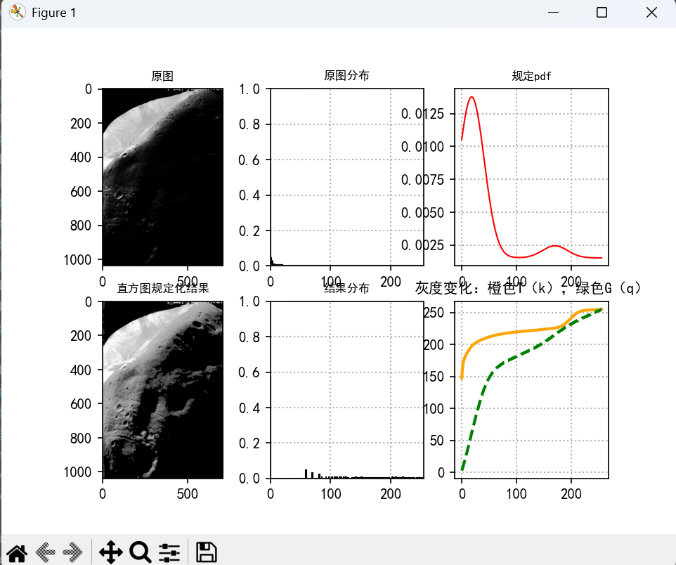
2)直方图规定化:多峰正态分布
import numpy as np
from PIL import Image
import matplotlib.pyplot as plt
from matplotlib.widgets import Slider
import matplotlib  # 导入主模块
matplotlib.use('TkAgg')  # 切换 Matplotlib 后端,解决 PyCharm 兼容性问题方法,切换到 Tkinter 后端(需保证 Python 安装了 tkinter,通常默认有),正确调用 use()

# 中文显示工具函数
def set_Chinese():
    # rcParams 本质是 matplotlib 主模块的全局配置字典
    matplotlib.rcParams["font.sans-serif"] =["SimHei"]
    matplotlib.rcParams["axes.unicode_minus"]=False

#获取图像的概率密度
def get_pdf(in_img):
    total = in_img.shape[0] * in_img.shape[1] #计算图像的总像素数
    return [ np.sum(in_img == i)/total for i in range(256) ] #求概率密度

#直方图均衡化(核心代码)
def hist_equal(in_img):
    #1、求原始图像的概率密度
    Pr = get_pdf(in_img)

    #2、构造输出图像(初始化成输入)
    out_img = np.copy(in_img)

    #3、执行“直方图均衡化”(执行累积分布函数变换)
    y_points = [] #存储点集,用于画图
    SUMk = 0 #累加值存储变量
    for i in range(256):
        SUMk = SUMk + Pr[i]  # SUMK 是从灰度 0 到灰度 i 的所有概率之和,范围在 0~1 之间。
        out_img[(in_img == i)] = SUMk * 255
        y_points.append(SUMk * 255)  # 构造绘制函数图像的点集,y_points 存储每个原始灰度 i 对应的新灰度值
    return out_img.astype("int32"), y_points

#生成均匀分布
def gen_eq_pdf():
    return [ 0.0039 for i in range(256)] #均匀概率密度1/256 = 0.0039

#生成多峰正态分布
#means 各峰均值
#stds 各峰标准差
#amp1 各正态分布幅值(和为1)
#bias 概率密度函数总体抬升量(若没有抬升量,容易造成图像过暗)
def gen_mul_norm_pdf(x,means,stds,ampl,bias):
    pdf = np.zeros([256,],dtype = float)
    for i in range(len(means)):
        pdf_temp = ampl[i]*np.exp(-(x-means[i])**2/(2*stds[i]**2))\
                    /(stds[i]*np.sqrt(2*np.pi))
        pdf = pdf + pdf_temp
    pdf = pdf + bias #总体抬升概率密度,避免出现零值
    pdf2 = pdf/np.sum(pdf) #由于做了抬升,所以要重新归一化
    return pdf2.tolist()


#构造目标图像的映射表(核心代码)
def gen_target_table(Pv):
    table = []
    SUMq = 0.
    for i in range(256):
        SUMq = SUMq + Pv[i]
        table.append(round(SUMq*255, 0)) #四舍五入
    return table

#直方图规定化(核心代码)
def hist_specify(in_img=None):
    #1、拿到目标图像规定的概率密度,并构造映射表
    #Pv = gen_eq_pdf()#均匀分布, 假设生成均匀分布的PDF(目标分布)
    Pv = gen_mul_norm_pdf(np.arange(0,256,1),[18,170],[23,23],[0.93,0.07],0.002)
    table = gen_target_table(Pv) # 目标分布的累积映射表
    print(table)

    #2、对原始图像做直方图均衡
    ori_eq_img, T_points = hist_equal(in_img) # 得到中间均衡化图像,ori_eq_img是原始图像经过直方图均衡化后的结果(灰度分布已被拉伸为近似均匀分布)

    #3、构造输出图像(初始化成输入)
    out_img = np.copy(ori_eq_img)

    #4、执行“直方图规定化”(做逆映射B'->B)
    mal_val = 0 #逆映射值初始化为0
    for v in range(256):
        if v in ori_eq_img: #存在于B’,如果当前灰度v存在于均衡化图像中
            if v in table: #存在于映射表,如果当前灰度v在目标映射表中存在对应值
    #拿到指定值最后出现的索引,python数组中的index下标只能拿到最小下标,多以要将table数组颠倒,再来拿下标,相当于拿到最大下标
                mal_val = len(table) - table[::-1].index(v)-1
            out_img[(ori_eq_img == v)] = mal_val #找不到映射关系时,取前一个映射值

    return out_img,T_points,table,Pv

if __name__ == "__main__":
    set_Chinese()
    # 以灰度值方式读取图像,
    gray_img = np.asanyarray(Image.open("../day4/planet.png").convert('L'))

    #对原图执行“直方图规定化”
    out_img,T_pts,G_pts,spec_hist = hist_specify(gray_img)

    #创建1个显示主体,并分成6个显示区域
    fig = plt.figure()
    ax1, ax2,ax3= fig.add_subplot(231), fig.add_subplot(232),fig.add_subplot(233)
    ax4, ax5,ax6 = fig.add_subplot(234), fig.add_subplot(235),fig.add_subplot(236)

    #窗口显示:原图,原图灰度分布、规定PDF,结果图像,结果图像灰度分析,对应变换函数
    # 窗口显示:原图
    ax1.set_title("原图", fontsize=8)
    ax1.imshow(gray_img, cmap='gray', vmin=0, vmax=255)

    # 窗口显示:原图灰度分布
    ax2.grid(True, linestyle=':', linewidth=1)
    ax2.set_title("原图分布", fontsize=8)
    ax2.set_xlim(0, 255)
    ax2.set_ylim(0, 1)
    ax2.hist(gray_img.flatten(), bins=255, density=True, color='black', edgecolor='black')

    # 窗口显示:规定PDF
    ax4.set_title("直方图规定化结果", fontsize=8)
    ax4.imshow(out_img, cmap='gray', vmin=0, vmax=255)

    # 窗口显示:结果图像灰度分析
    ax5.grid(True, linestyle=':', linewidth=1)
    ax5.set_title("结果分布", fontsize=8)
    ax5.set_xlim(0, 255)
    ax5.set_ylim(0, 1)
    ax5.hist(out_img.flatten(), bins=255, density=True,color='black',edgecolor='black')

    #绘制规定概率密度函数
    ax3.set_title("规定pdf", fontsize=8)
    ax3.grid(True, linestyle=':', linewidth=1)
    ax3.plot(np.arange(0, 256, 1), spec_hist, color='r', lw=1)

    #窗口显示:绘制对应的灰度变换函数
    ax6.set_title("灰度变化:橙色T(k),绿色G(q)", fontsize=10)
    ax6.grid(True, linestyle=':', linewidth=1)
    ax6.plot(np.arange(0,256,1),T_pts,'-',color='orange',lw=2)
    ax6.plot(np.arange(0,256,1),G_pts,'k--',color='green',lw=2)

    plt.show()
运行结果
四、tips
在学习过程中,敲一遍代码能够加深对于数字图像处理的理解。
比如,直方图均衡化,是把集中型直方图变为均匀型直方图,为什么做了直方图均衡化之后,没有改变图像的形状?
直方图均衡化的本质:直改变“灰度值”,不改变“像素位置”,图像的“形状”由像素的空间位置关系决定(例如一个矩形的形状由其边缘像素的坐标排列决定),而直方图均衡化的操作是保持像素的位置不变,只是灰度值被替换。
改变像素的位置:让图像中每个像素的坐标发生移动---原本在图像(x,y)位置的像素,被挪到(x‘,y’)的位置,最终会改变图像中物体的形状大小位置。例如:图像平移:把整张图向右移动100个像素,向下移动50个像素,物体的位置变了,但是形状没变
改变像素位置:动的是”像素在哪“(坐标),会影响图像的形状大小位置;
直方图均衡化:动的是“像素是什么灰度”(数值),像素的坐标完全不变、所以形状、结构都不变,只变明暗对比。
所以,图像成像的原理是:图像 = 像素的位置(坐标) + 像素的数值(灰度 / 颜色),两者共同决定了我们看到的画面。不能把像素的位置和数值混淆!